Update: The dhang is now available for preorder, and you can join a workshop to build it yourself!
Feedback from first user testing of the dhang digital hand drum was that the latency was too high. How did we bring it down to a good level?
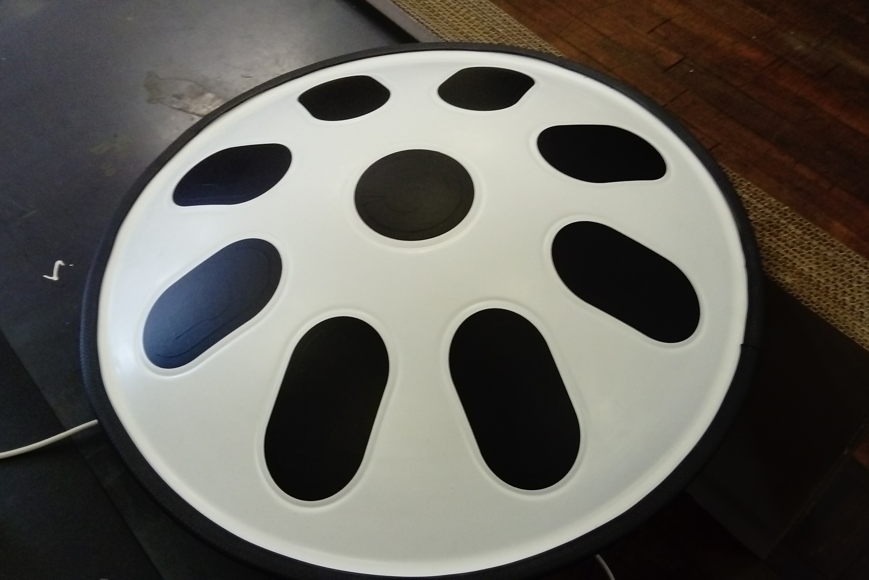
dhang: A MIDI controller using capacitive touch sensors for triggering. An Arduino board processes the sensor data and sends MIDI notes over USB to a PC or mobile device. A synthesizer on the computer turns the notes into sound.
Testing latency
For an interactive system like this, what matters is the performance experienced by the user. For a MIDI controller that means the end-to-end latency, from hitting the pad until the sound triggered is heard. So this is what we must be able to observe in order to evaluate current performance and the impact of attempted improvements. And to have concrete, objective data to go by, we need to measure it.
My first idea was to use a high-speed camera, using the video image to determine when pad is hit and the audio to detect when sound comes from the computer. However even at 120 FPS, which some modern cameras/smartphones can do, there is 8.33 ms per frame. So to find when pad was hit with higher accuracy (1ms) would require using multiple frames and interpolating the motion between them.
Instead we decided to go with a purely audio-based method:
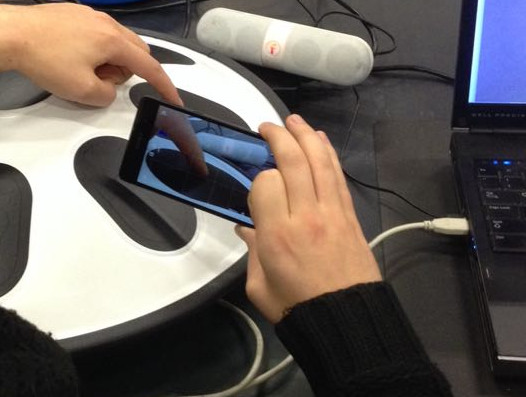
Test setup for measuring MIDI controller end2end latency using audio recorded with smartphone.
- The microphone is positioned close to the controller pad and the output speaker
- The controller pad is tapped with the finger quickly and hard enough to be audible
- Volume of the output was adjusted to be roughly same level as sound of physically hitting the pad
- In case the images are useful for understanding the recorded test, video is also recorded
- The synthesized sound was chosen to be easily distinguished from the thud of the controller pad
To get access to more settings, the open-source OpenCamera Android app was used. Setting a low video bitrate to save space, and enabling macro-mode for focusing close objects easier. For synthesizing sounds from the MIDI signals we use LMMS, a simple but powerful digital music studio.
Then we open the video in Audacity audio editor to analyze the results. Using Effect->Amplify to normalize the audio to -1db makes it easier to see the waveforms. And then we can manually select and label the distance between the starting points of the sounds to get our end-to-end latency.
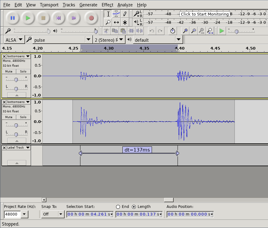
Raw sound data, data with normalized amplitude and measured distance between the sound of tapping the sensor and the sound coming from speakers.
How good is good enough?
We now know that the latency experienced by our testers was around 137 ms. For reference, when playing a (relatively slow) 4/4 beat at 120 beats per minute, the distance between each 16th notes is 125 ms. In the following soundclip the kickdrum is playing 4/4 and the ‘ping’ all 16 16th notes.
So the latency experienced would offset the sound by more than one 16th note! We can understand that this would make it tricky to play.
For professional level audio, less than <10 ms is a commonly cited as the desired performance, especially for percussion. From Action-Sound Latency: Are Our Tools Fast Enough?
Wessel and Wright suggested that digital musical
instruments should aim for latency less than 10ms [22]
Dahl and Bresin [3] found that in a system
with latency, musicians execute their gestures ahead of the
beat to align the sound with a metronome, and that they
can maintain synchronisation this way up to 55ms latency.
Since the instrument in question is going to be a kit targeted at hobbyists/amateurs, we decided on an initial target of <30ms.
Sources of latency
Latency, like other performance issues, is a compounding problem: Each operation in the chain adds to it. However usually a large portion of the time is spent in a small parts of the system, so an important part of optimization is to locate the areas which matter (or rule out areas that don’t).
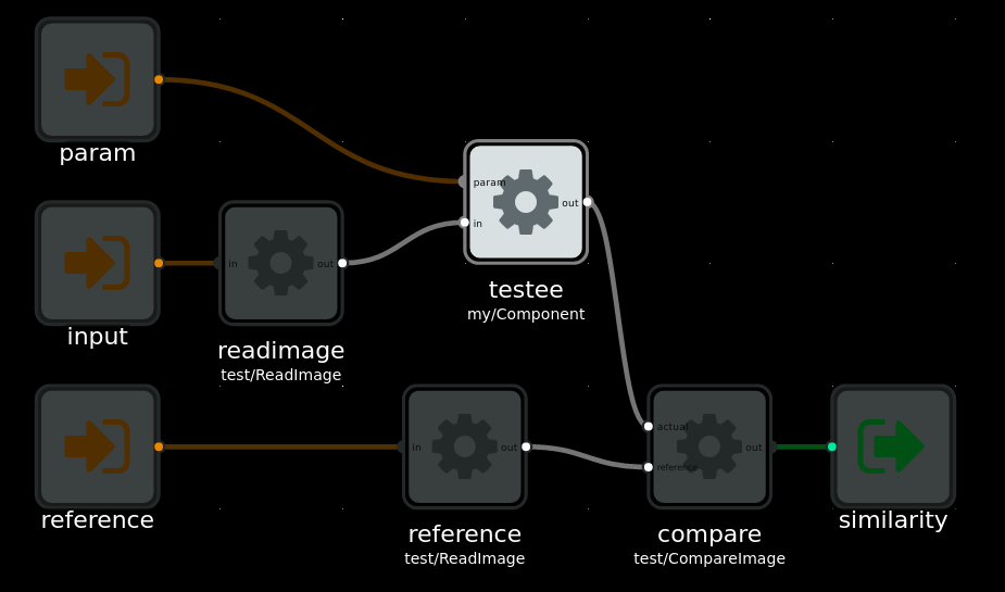
For the MIDI controller system in question, a software-centric view looks something like:
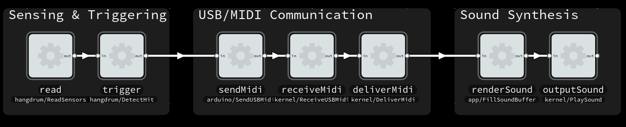
A functional view of the system and major components that may contribute to latency. Made with Flowhub
There are also sources of latency outside the software and electronics of the system. The capacitive effect that the sensor relies on will have a non-zero response time, and it takes time for sound played by the speakers to reach our ears. The latter can quickly be come significant; at 4 meters the delay is already over 10 milliseconds.
And at this time, we know what the total latency is, but don’t have information about how it is divided.
With simulation-hardened Arduino firmware
The system tested by users was running the very first hardware and firmware version. It used a an Arduino Uno. Because the Uno lacks native USB, a serial->MIDI bridge process had to run on the PC. Afterwards we developed a new firmware, guided by recorded sensor data and host-based simulation. From the data gathered we also decided to switch to a more sensitive sensor setup. And we switched to Arduino Leonardo with native USB-MIDI.
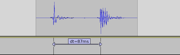
Latency with new firmware (with 1 sensor) was reduced by 50 ms (35%).
This firmware also logs how long each sensor reading cycle takes. It was under 1 ms for the recorded single-sensor setup. The sensor readings went almost instantly from low to high (1-3 cycles). So if the sensor reading and triggering takes just 3 ms, the remaining 84 ms must be elsewhere in the system!
Low-latency audio, a hard real-time problem
The two other main areas of the system are: the USB/MIDI communication from the Arduino to the PC, and the sound synthesis/playback. USB MIDI should generally be relatively low-latency, and it is a subsystem which we cannot influence so easily – so we focus first on the sound aspects.
Since a PC must be able to do multi-tasking, audio is processed in chunks: a buffer of N samples. This allows some flexibility. However if processing is interruptedfor toolong or too often, the buffer may not be completely filled. The resulting glitch is usually heard as a pop or crackle. The lower latency we want, the smaller the buffer, and the higher chance that something will interrupt for too long. At 96 samples/buffer of 48kHz samplerate, each buffer is just 2 milliseconds long.
With JACK on on Linux
I did the next tests on Linux, since I know it better than Windows. Configuring JACK to 256 samples/buffer, we see that the audio configuration does indeed have a large impact.
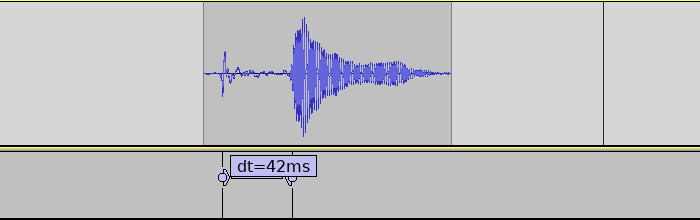
Latency reduced to half by configuring Linux with JACK for low-latency audio.
With ASIO4ALL on Windows
But users of the kit are unlikely to use Linux, so a solution that works with Windows is needed (at least). We tried all the different driver options in LMMS, switching to Hydrogen drum machine, as well as attempting to use JACK on Windows. None of these options worked well.
So in the end we tried going with ASIO, using the ASIO4LL replacement drivers. Since ASIO is proprietary LMMS/PortAudio does not support it out-of-the-box. Instead you have to manually replace the PortAudio DLL that comes with LMMS with a custom one 🙁 *nasty*.
With ASIO4ALL we were able to set the buffer size as low as 96 samples, 2 buffers without glitches.
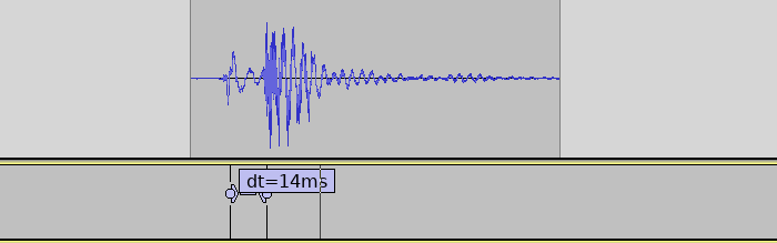
ASIO on Windows achieves very low latencies. Measurement of single sensor.
Completed system
Bringing back the 8 other sensors again adds around 6 ms to the sensor reading, bringing the final latency to around 20ms. There are likely still possibilities for significant improvements, but the target was reached so this will be good enough for now.
A note on jitter
The variation in latency of a audio system is called jitter. Ideally a musical instrument would have a constant latency (no jitter). When a musical instrument has significant amounts of jitter, it will be harder for the player to compensate for the latency.
Measuring the amount of jitter would require some automated tools for the audio analysis, but should otherwise be doable with the same test setup.
The audio pipeline should have practically no variation, but the USB/MIDI communication might be a source of variation. The CapacitiveSensor Arduino library is known to have variation in sensor readout time, depending on the current capacitance of the sensor.
Conclusions
By recording audible taps of the sensor with a smartphone, and analyzing with a standard audio editor, one can measure end-to-end latency in a tactile-to-sound instrument. A combination of tweaking the sensor hardware layout, improving the Arduino firmware, and configuring PC software for low-latency audio was needed to aceive acceptable levels of latency. The first round of improvements brought the latency down from an ‘almost unplayable’ 134 ms to a ‘hobby-friendly’ 20 ms.
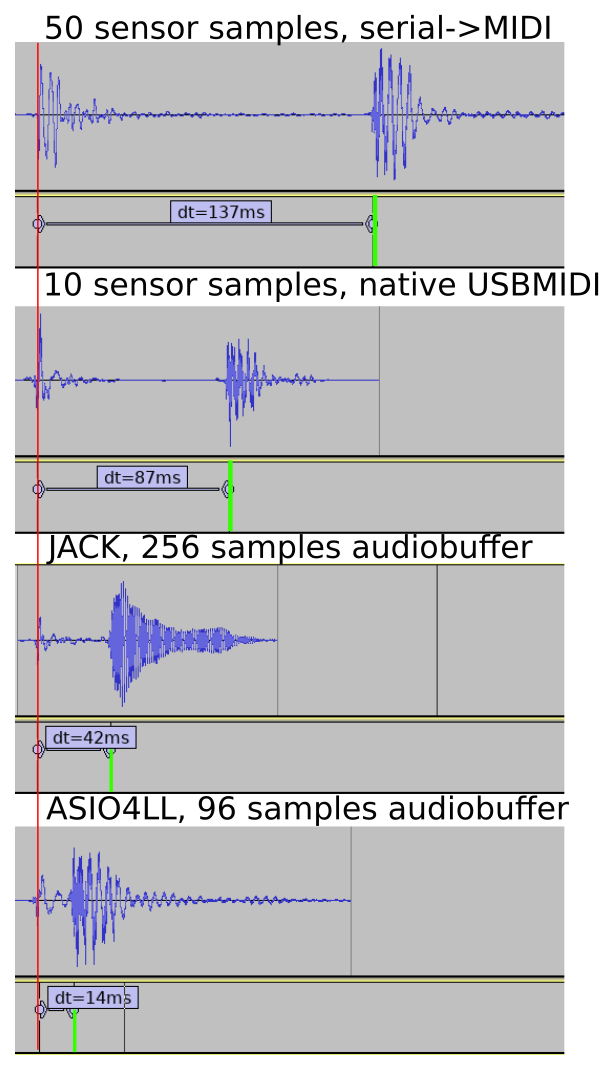
Comparison of latency betwen the different configurations tested.