Back in 2018, during my master in Data Science, I started the emlearn project – implementing classic Machine Learning models designed to run on microcontrollers and embedded devices (aka “TinyML”). Back then, the primary purpose was to learn the ins and outs of these algorithms, to make sure I really understood them well. Thinking about how the algorithms can be implemented efficiently in terms of RAM usage, storage space and CPU time is excellent for that purpose. But I always made sure to keep the code at production-quality, with a decent set of automated tests.
emlearn in use
Fast-forward 5 years, and emlearn has actually been used in a wide range of real-world projects, which is fantastic. Due to the open-source nature, everyone can just download it and use it for whatever they want – so there are probably many uses we will never hear about. And that is fine 🙂 But, there are some uses that I do know of. So here is a small selection of some of the projects using emlearn.
These projects highlight some of the typical characteristics for projects where emlearn is a good fit. Sensor data is analyzed on-device using a combination of Digital Signal Processing and Machine Learning. The extracted information is a low rate data-stream which can then be transmitted wirelessly. All of this can be done on low-cost hardware using general-purpose microcontrollers. Many tasks can also be done at low-power and run on battery.
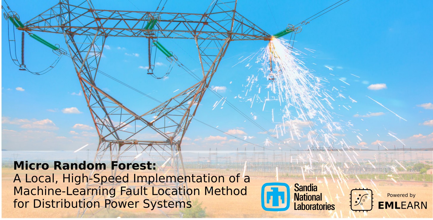
Researchers from Sandia National Laboratories developed a system to identify the origin of faults in the power grid. When an abrupt fault occurs in a power transmission line, this causes a wave that propagates along the line. The wave is influenced by the electrical characteristics of the line as it travels along to other locations in the grid. The researchers used a combination of Digital Signal Progressing and Random Forest classifier to analyzes the signature of an incoming wave, and determines where the fault originated. They tested the system by injecting faults in a simulated model of a grid, and then ported the procedure to a DSP board from Texas Instruments.
Being able to automatically locate failures that occur in grid power lines is key to being able to dispatch maintenance crews to the right place, and could enable quicker recovery times after failures.
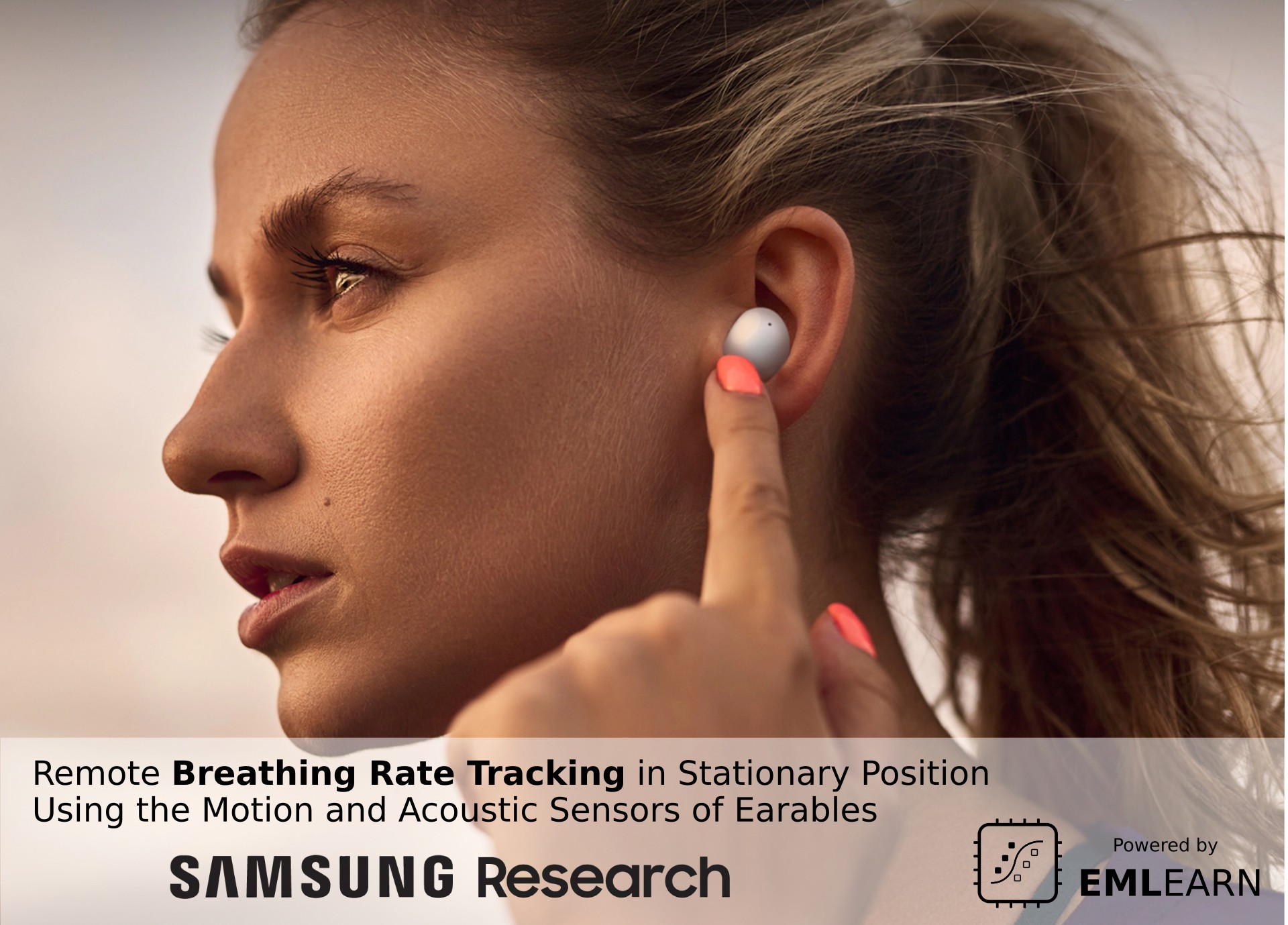
Researchers at Samsung used a combination of motion data from the accelerometer and sound data from the microphone on Samsung Galaxy earbuds to estimate breathing rate. First, breathing rate estimation is attempted using the accelerometer. If no estimation can be made, then the audio microphone data is used to estimate breathing rate. This multi-modal approach handles a wide range of cases, which they tested both in a laboratory and home setting. The battery consumption was low enough that the measurements could run continuously.
This kind of technology could be especially useful for people with respiratory diseases, who often need to check their breathing rate to manage and quantify their lung condition.
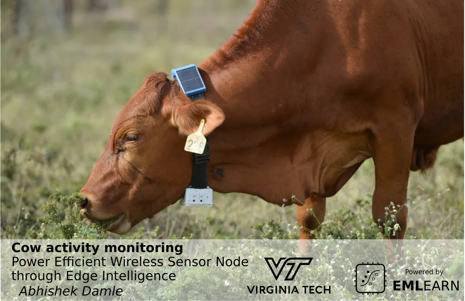
Abhishek Damle, who was a master student at Virginia Tech in 2022, developed a battery-powered sensor that tracks cattle activity. The sensor is mounted on the cow’s halter, and uses a low-power accelerometer to sense motion. A decision tree is used to classify whether the cow is lying/walking/standing/grazing/ruminating. The detected activity is then transmitted LoRaWAN to a central location. They estimate that doing the machine learning on-sensor it consumes under 1 mW, which is 50 times less than if transmitting the raw data.
The activity data can be used to detect abnormal behavior in a cow, which can indicate health issues or other problems.
Recent developments
Classification, regression and anomaly detection
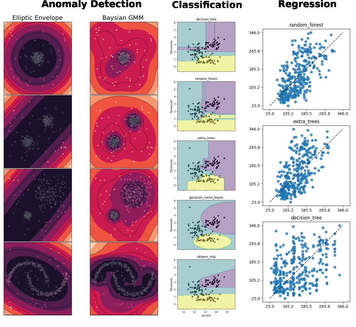
emlearn allows converting scikit-learn and Keras models trained in Python into efficient and portable C code. The first versions of only supported classification. Over the last years, we have also added support for regression and anomaly/outlier detection for a range of models.
Examples of outputs for some of the models supported by emlearn, in different types of ML tasks
Improved documentation
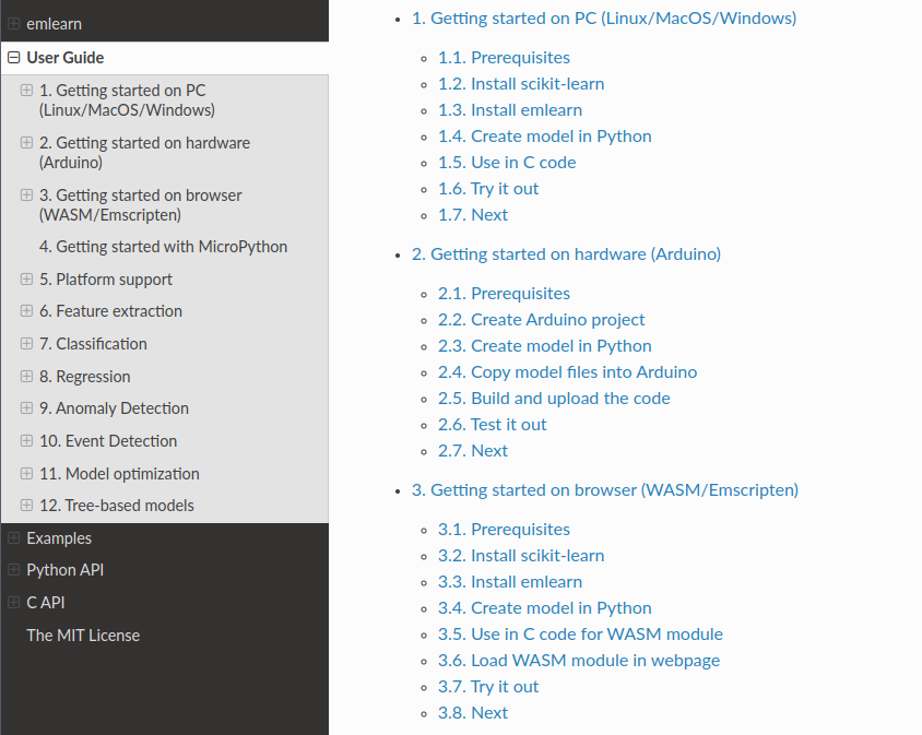
To facilitate further usage, I decided to do a pass to improve the documentation this summer. Now there is more detailed documentation for Getting Started, that covers setting up and running the first model – be it on your PC, on Arduino, or running in a Web browser. There are also task-oriented pages in the user-guide – covering Classification, Regression, Anomaly Detection, Event Detection (for now).
emlearn documentation now has a User Guide, C API reference, Python API reference and Examples
MicroPython support
Whereas C is the lingua franca for embedded/firmware engineers, Python is the lingua franca for Data Scientists and Machine Learning Engineers. emlearn itself is written in portable C99, and makes it easy to train in Python (on computer) and deploy to C (on device). This is practical, but for some users and applications it could be even nicer to do also the device code in Python. This is now made easy with emlearn-micropython.
The MicroPython project is a Python (3.x) implementation designed for microcontrollers. It is around 10 years old by now, and has a good level of maturity. It is a very efficient and compact Python implementation, and runs on 32-bit devices with at least 256k of code space and 16k of RAM.
The emlearn-micropython are released as .mpy modules, which can be added to an existing board by copying it over USB/serial/WiFi. No rebuilding or flashing of the firmware needed! This uses the dynamic native modules feature in MicroPython. This is really quite magical, and lets us realize a workflow which has the convenience of Python, and the efficiency of C.
Example code for host
# Train a model using scikit-learn
estimator = RandomForestClassifier(n_estimators=3, max_depth=3, max_features=2, random_state=1)
estimator.fit(X, y)

# Convert model using emlearn
cmodel = emlearn.convert(estimator, method='inline')

# Save as loadable .csv file
cmodel.save(file='xor_model.csv', name='xor', format='csv')
Example code for device
import emltrees
import array

model = emltrees.new(5, 30) # ensemble of up to 5 trees and 30 decision nodes

# Load a CSV file with the model
with open('xor_model.csv', 'r') as f:
    emltrees.load_model(model, f)

# run inference with the model
examples = [
    array.array('f', [0.0, 0.0]),
    array.array('f', [1.0, 1.0]),
    array.array('f', [0.0, 1.0]),
    array.array('f', [1.0, 0.0]),
]
for ex in examples:
    result = model.predict(ex)
    print(ex, result)
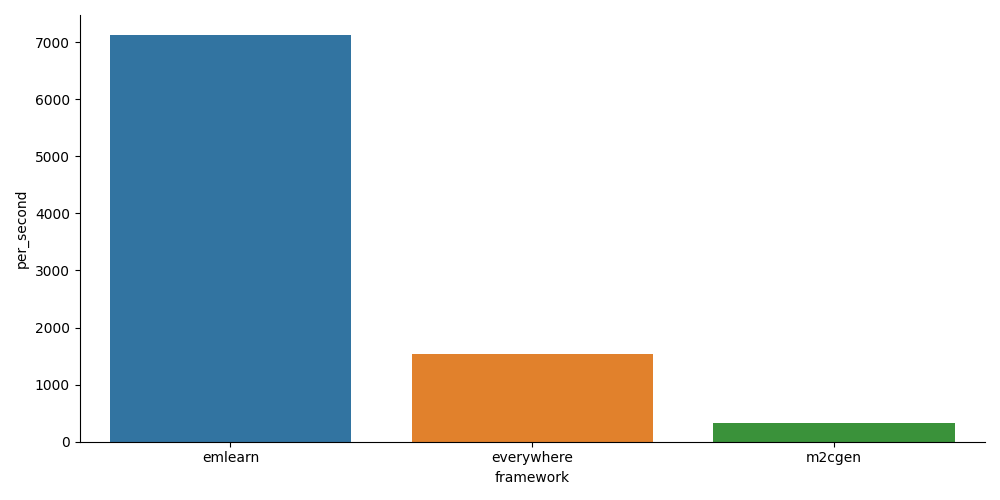
There are some existing projects that allow to generate (Micro)Python code for ML models, such as m2cgen and everywhereml. But while MicroPython is a pretty efficient Python, a C implementation should still be able to do better. To test this, I ran some quick benchmarks. These were performed on a RP2040, an affordable and popular ARM Cortex M0 chip.
Inference speed comparison of emlearn-micropython compared to other frameworks. Y axis is the number of samples per second (higher is better).
As expected, the emlearn approach is many times faster than pure-Python based approaches. This could be further increased by enabling fixed-point/integer support in emlearn.
The TinyML wave has only just begun
emlearn is a library for Machine Learning on microcontrollers and embedded systems – often referred to as TinyML. There are over 20 billion microcontrollers shipped every year. From 2022 it is estimated that over 2 billion of these are TinyML devices, up from 15 million in 2019[1]. So it is still very early days for this field. And it will be very interesting to see where emlearn goes in the next 5 years.
At EuroPython 2019 in Basel I gave an introduction to the use of modern machine learning for audio classification. It was very well received, both at the event and the video recording afterwards. The full video recording can be found here (YouTube).
Below I provide a transcript of the presentation, for those who prefer to read instead of looking at a video.
Introduction
[chair]
Welcome to the session.
Jon Nordby is a maker and full-stack IoT developer.
He successfully defended his master’s thesis in Data Science two weeks ago and he’s now embarked on an IoT startup called Soundsensing.
Today he’ll talk to us about a topic related to his thesis: Audio classification with machine learning.
[presenter]
Hi thank you.
So, audio classification is not such a popular topic as for instance image classification or a natural language processing.
So I’m happy to see that there’s still people in the room and interested in this topic.
About me
So first a little about me. I’m an Internet of Things specialist.
Have background in electronics from nine years ago.
Worked a lot as a software engineer, because electronics is mostly software these days or a lot of software.
And then I went to do a Masters in Data Science because IoT to me is the combination of
electronics (sensors especially),
software (you need to process the data),
and data itself – transform sensor data into information that is useful.
Now I’m consulting on IoT and machine learning and I’m also CTO of Soundsensing.
We deliver sensor units for noise monitoring.
About the talk
In this talk my goal (we’ll see if we get there), is that you as a machine learning practitioner, without necessarily prior experience in sound processing, can solve a basic Audio Classification problem.
We’ll have an introduction about digital sound very briefly.
And then we’ll go through a basic audio classification pipeline.
And then some tips and tricks for how to kind of go little bit beyond that basic.
And then I’ll give some pointers to more information.
The slides and a lot of my notes on machine hearing, in general little bit broader than audio classification, is on this github: https://github.com/jonnor/machinehearing/
Applications
There are some very well recognized subfields of audio, speech recognition is one of them.
And for instance there you have as a classification task you have keyword spotting, so: "Hey Siri" or "OK Google".
And in music analysis you also have many tasks, genre classification for instance can be seen as a simple audio classification task.
We’re gonna keep it mostly on the general levels: we’re not gonna use a lot of speech or music specific domain knowledge.
We still have examples across a wide range of things, I mean anything you can do with hearing as a human you we can get close to (on many tasks at least) with machines today.
In ecoacoustics you might wanna analyze bird migrations using sensor data to see their patterns.
Or you might want to detect poachers in protected areas to make sure that no one actually is going around shooting where there should be no gunshots.
It’s used in quality control in manufacturing. Especially because you don’t have to go into the equipment or the product under test, you can listen it to it from the outside.
For instance used for testing your electrical car seats they check that all motors run correctly.
In security it’s used to help monitor large amounts of CCTVs by also analyzing audio.
And in medical for instance you could detect heart murmurs which could be indicative of a heart condition.
Background
Digital sound
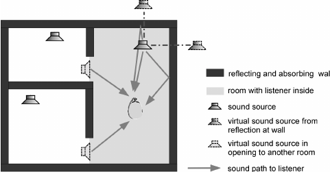
First thing to that is important is that sound is almost always, or basically always, a mixture.
Because sound, I mean, it will move around the corner, unlike image for instance.
And you will always have sound coming from multiple placee.
It will also transport in the ground and be reflected by a wall.
And all these things makes it so you always have multiple sound sources:
The source of interest and then always other sound sources (noise).
Audio Aquisition
Physically we have a sound as its variation in air pressure.
We go through a microphone to converted to electrical voltage,
an Analog-to-Digital converted (ADC) and then we have a digital waveform – which is what we will deal with.
As digital audio, it’s quantized in time for instance with the sampling rate and amplitude.
We usually deal with mono primarily with one channel when we do Audio Classification.
There are some methods around stereo but not widely adopted, and also more channels.
We typically use uncompressed formats, it’s just the safest.
Although you in real life situation you might also have compressed data,
which can have artifacts and so on that might influence your model.
Spectrograms
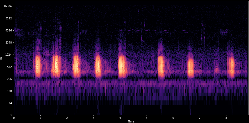
So after we have a waveform we can convert it in a spectrogram.
And this is in practice a very useful representation,
both as a human for understanding (what is this sound) and for the machines.
To use this one example, is a frog croaking like / r / r / r.
Very periodically, with a little gap.
And then it’s hard to see but in top in a higher level there is some cicadas that are going as well.
This allows us to both see the few frequency representation and the patterns across time.
And together often this allows you to separate different sound sources from your mixture.
Environmental Sound Classification
So we’ll go through a practical example just to keep it kind of hands-on. Environmental Sound Classification.
Given a signal of environmental sounds, these are everyday sounds that are around in the environment.
For instance it can be out outdoors: Cars, children and so on.
It’s very widely researched. We have several open data sets that are quite good. AudioSet is several I think tens of thousands or even hundreds of thousands of samples.
And in 2017 we’ve reached roughly human level performance (only one of these data sets, ESC-50 , has an estimate for what is human level performance) but we seem to have surpassed enough.
Urbansound8k dataset
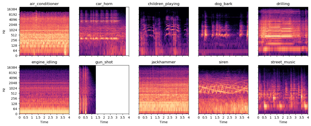
And one nice data set is the Urbansound8k which has ten classes of 8k samples.
They’re roughly 4 seconds long and 9 hours total and state of the art here is around 80 percent (79 to 82) of accuracy.
Here we have some spectrograms and these are the easy samples.
This data set has many challenging samples where the sound of interest is very far away and hard to detect, and these ones are easy.
So you see the siren goes like very up and down and jackhammers and drilling have very periodic patterns.
So how can we detect this using a machine learning algorithm in order to output these classes?
A simple Audio Classification pipeline
I will go through a basic audio pipeline, and skipping around like 30 to 100 years of history of audio processing, kind of going straight to what is now the typical way of doing things.
And it looks something like this.
Overview
So first in the input we have our audio stream.
It’s important to realize that of course audio has time related to it so it’s more like a video than to an image.
And in practical case scenario might you do real-time classification so this might be a infinite stream that just goes on and on.
So it’s important for that reason and for also the Machine Learning to divide the stream into small or relatively small analysis windows that you will actually process.
However you often have the mismatch between how often you have labels for your data versus how often you actually want a prediction.
This is known as weak labeling.
I won’t go much into it but so in the Urbansound8k it’s for sound 4 seconds sound snippet so that’s what kind of are we’re given and this curated data set.
However it’s usually beneficial to use smaller analysis windows to reduce the dimensionality of the machine learning algorithm.
So the process goes that we will divide the audio into these segments, it will often use overlap.
And then we’ll convert it into a spectrogram and we’ll use a particular type of spectrogram called a Mel-spectrogram which been shown to work well.
And then we’ll pass that frame or features from the spectrogram into our classifier and it will output the classification for that small time window.
And then because we have labels per 4 seconds we’ll need to do an aggregation in order to come up with the final prediction for these four seconds, not just for this one little window.
Yeah we’ll go through these steps now.
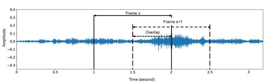
Overlap of analysis windows
So first analysis we notice I mention we often use overlap.
Overlap is sometimes specified in two different ways: one is an overlap percentage.
Here we have 50% overlap, so that means that we’re essentially classifying parts of the or we’re classifying every piece of the other stream twice.
So we could have even more overlap people maybe a 90 percent overlap then we’re classifying it 10 times.
And that gives the algorithm multiple viewpoints on this audio stream, and makes it easier to catch the sounds of interest.
Because the model might in training, might have learned to prefer a certain sound to appear in a certain position inside this analysis window.
Overlap is a good way of of working with that.
Mel-spectrograms preprocessing
so a mission we used a specific type of spectrogram.
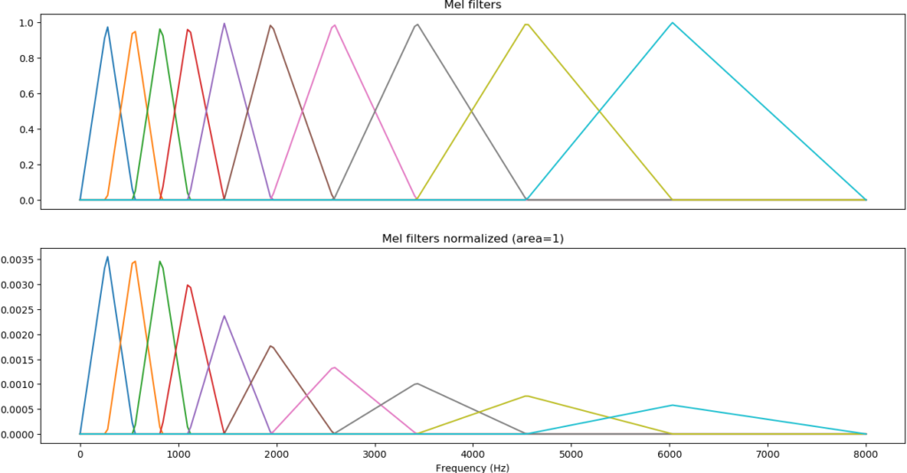
So the spectrogram is usually processed with those called Mel-scale filters these are inspired by the human hearing.
Our ability to differentiate sounds of different frequencies reduce is reduced as frequencies to get higher.
So low sounds were able to detect small frequency of variations however high pitched sounds we need large frequency variations towards.
And by using this kind of filters on the spectrogram we obtain the representation is some more similar to our ears.
But more importantly it’s a smaller representation for a machine learning model, and also you’ll be able to merge kind of related data in in two consecutive bins for instance.
So when you’ve done that it looks something like this.
On the top is a normal spectrogram and you see kind of a lot of small details.
The bottom one we’ve we started the Mel filters at 1000 Hertz.
This is bird audios which is quite high pitched, a lot of chirps up and down.
And in the third one we’ve with normalized the earth.
We usually use log-scale compression because sound has a very large dynamic range.
So sounds that are faint versus sounds that are very loud for the human ear is a factor of 1000 or a factor of 10,000 in energy difference.
So when you’ve normalized log-scaled applied the spectrum and normalized you look at something like the image below.
So in Python code this picture shows the processing.
I’m not gonna go through all this in detail, we have an excellent library called librosa which is great for just loading and loading the data and doing basic feature pre-processing.
Also some of the deep learning frameworks have their own Mel-spectrogram implementations that you may also.
Normalizing across sample or window
But there is a general thing in streaming.
So when people analyze audio they often apply normalization learned from the mean for instance across their whole samples for four seconds in this case, or from their whole data set.
That can be hard to to apply when you have a continuous audio stream which has for instance changing volume and so on.
So what we usually do is to normalized per frame so the hope is that you have enough information in our roughly one second of the data in order to do a this normalization.
And doing normalization like this has some interesting consequences when there is no input.
Because what happens is if you have no input to your system, probably you’re gonna blow up all the noise.
So your sometimes need to exclude very low energy signals from being classified.
Just like little practical tip.
Convolutional Neural Network
So Convolutional Neural Networks, they’re hot.
Who here has basic familiarity, at least gone through a tutorial or read a blog post about image classification and CNN’s?
Yeah that’s quite a few.
So CNN’s are the best in class for image classifications.
Spectrograms are image-like audio representation, they have some differences, so a question is (or maybe it was): will CNN’s work well on spectrograms?
Because that would be interesting and the answer is… yes.
This been researched quite a lot, and this is great because there is a lot of tools, knowledge, experience and pre-trained models for image classification.
So being able to reuse those in the audio domain, which is not such a big field, is a major major win.
So you’ll see a lot of the research lately is, it can be a little bit boring in audio classification research, because a lot of it is like taking one year ago image classifying tools and applying them, and seeing whether it works.
It is however a little bit surprising that this actually works because the spectrogram has frequency on the y-axis (typically it’s shown that way) and time on the other axis.
So a movement or a scaling in this space doesn’t mean the same as in an image.
You know an image if I have my face inside an image doesn’t matter where my face appears.
If you have a spectrogram and you have certain sound it’s like a chirp up and down, if you move that up in frequency or down, at least if you move it a lot, it’s probably not the same sound anymore.
It might go from a human talking to a bird, the shape might be similar but the position matters.
So it’s a little bit surprising that this works, but it does seem to do really well in practice.
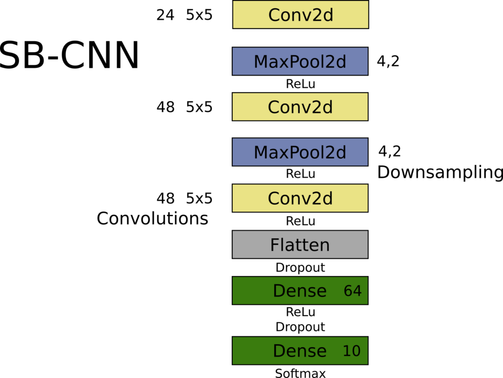
SB-CNN
So this is one model that does well on Urbansound.
And one thing you’ll note compared to a lot of image models is that it’s quite simple, I mean relatively few layers. This is smaller than or the same kinda size as LeNet5.
And there are three convolutional blocks followed by Mike and with max pooling between the two first blocks.
And that’s, you know, the standard kind of CNN architecture.
This one using five by five instead of two or three kernels, doesn’t make much of a difference you could stack another layer and do the same thing.
And we flatten and then we use a fully connected layer.
From 2016 and still is one is like close to state-of-the-art on this dataset, Urbansound8k.
If you are training CNN from scratch on audio data, start with a simple model.
I mean there’s no usually no reason to start with say VGG16 with 16 layers and millions of parameters,
or even MobileNet or something like that.
You can usually go quite far with with this kind of simple architecture – a couple of convolutional layers.
So in case for example this could look something like this.
Where we have our individual kind of blocks. Convolution, Maxpooling, ReLu non-linearity.
Same for the second one and our full classification at the end the full connected layers.
So this is our classifier.
We will pass the spectrogram analysis window through this,
and it will give us a prediction for which class it was among the classes in Urbansound.
Aggregating analysis windows
And then we need to aggregate these individual windows, and there are multiple ways of doing this.
You could do simplest kind of thing to think about is to do majority voting.
So if we have ten windows over four second spectrum we could do the predictions,
and then just say okay the majority (most common) class wins. That works rather well.
But it’s not differentiable, and so it is done as post-processing.
And you’re making very rough predictions on each on a step.
So mean mean pooling or global average pooling across those analysis windows usually does a little bit better.
And it’s nice with deep learning frameworks is that you can also have this as a layer so for instance in Keras you have the TimeDistributed layer.
Which is there’s sadly extremely a few examples of online.
It’s not that hard to use but it took me a while it to to figure out how they do it.
So we apply a base model, which is in this case the input to this function.
We pass it to the TimeDistributed layer and which essentially it will use a single instance of your model, so it’ll share the weights for all these steps for all the analysis windows.
And then it will just run in multiple times when you do the prediction step and then it will global average pooling over these predictions.
So here we’re averaging predictions you can also you can also do more advanced things where you would for instance average your feature representation and then do a more advanced classifier on top of this.
But this was called probabilistic voting quite often in literature, when you do this mean pooling.
That allows us so this will give us a new model which is what will take not single in analysis windows, which will take a set of analysis windows typically corresponding to our 4 seconds with for example 10 windows.
Demo
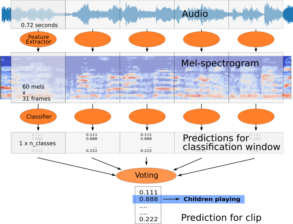
So if you do this and a couple more tricks from my thesis you can have a system working like this demo.
So this has, in addition to building model and so on which I’ve gone through,
we’re also deploying to a small microcontroller using the vendor provided tools that converts a Keras model.
And so that’s kind of roughly standard things, so I don’t go into it here.
So little demo video (if we have sound).
Here is Children playing.
Thing is basically what we do also here is we threshold the prediction. So if no prediction is good we’ll consider it unknown.
And this is also important in practice because sometimes you have out of class data.
This is Drilling.
Or this actually the the sample I found said jackhammer. Jackhammer is actually another class.
And really they are to my ear hard to distinguish sometimes and the model can also struggle with it.
There is Dog Barking.
And so in this case all the classification happens on the small sensor unit which is what I focused on in my thesis.
Siren
The model actually it didn’t get the first part of the siren. Only the undulating part later.
So actually these samples are not from the Urbansound dataset which I’ve trained out.
So they’re "out of domain" samples, which is generally a much more challenging.
Yes that’s it for demo.
If you want to know more about doing sound classifications on these sensor units you can get my full thesis.
Both the report and the code is there.
Tips & Trick
Some tips and tricks.
So we’ve covered the basic audio processing pipeline, the modern one, and that will give you results and generally quite good results with the modern CNN architecture.
And there are some tips and tricks especially in practice where when you are having a new problem:
You’re not researching an existing data set, your data sets are usually much smaller and it’s quite costly and tedious to annotate all the data
And so here are some tricks for that.
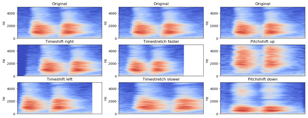
Data Augmentation
First one is data augmentation.
This is well known from from other deep learning applications, especially image processing.
And the augmentation can be done on audio can be done either in the time domain or in the spectrogram domain. And in practice it both seem to work work fine.
So here are some examples of common common augmentations.
The most common and possibly most important is to do time shifting.
So remember that I said that when you classify an analysis window we may one second you know the sounds of interest there.
And what the individual convolution kernel sees what might be very short.
If you have bird chirps they’re like and those are you know maybe 100 milliseconds max or maybe in 10 milliseconds so they they occupy very little space in that image that the classifier sees.
But it’s important that it’s able to classify classify it no matter where inside this analysis window it appears.
So time shifting simply means that you shift your samples in time forward and backward (left and right).
And that gives them you know that I would have seen that okay bird chirps can appear you know many places in time at any place in time and it doesn’t make a difference to the classification.
So this is by far the most important one and you can usually go quite far with just time shifting.
If you do want precise location of your event, so you want to have a classifier that can tell when did chirps appear.
In the 100 millisecond range instead of just that there was birds in this 4-10 seconds audio then you might not want to do time shifting.
Because you might want to have the output based on that the sound always occurs in the middle of the window.
But then you need to your labeling needs to to respect that.
Time stretching.
So many sounds you know if I speak slowly or I speak very fast its it’s the same, you know it’s the same meaning, it’s the same certainly the same class it’s both speech.
So time stretching is also very very efficient to capture such variations.
And also pitch shifting. So if if I’m speaking with low voice or a high-pitched voice you know, it’s still the same kind of information.
And the same carries in in you know for general sounds, at least a little bit, so a little bit of time shift you a pitch shift you can accept, but a lot of big shift might kind of bring you into new class.
For instance the difference between human speech and and bird chirps might be a big pitch shift.
So so you might want to limit how much you pitch shift.
Typical augmentation settings here is like maybe 10 to 20 percent on time shift and pitch.
You can also add noise.
This is also quite efficient especially if you do know that you have variable amount of noise.
Random noise works okay you can also sample.
There’s lot of repositories of basically noise, so you’ll mix in noise with your signal and classify that.
Mix-up is an interesting data augmentation strategy that makes these two samples like by a linear combination of the two and actually adjusts the labels accordingly.
And that has been shown to work really well also in combination with other augmentation techniques on the audio.
Transfer learning
So yes we can basically apply CNN’s to audio, and with the standard kind of image type architecture. This means that we can do transfer learning from image data.
So of course image data has, I mean is, significantly different from from spectrograms.
I mentioned the frequency axis and so on.
However the some of the base operations that are needed you need to detect edges you need to detect diagonals,
you need to detect patterns of edges and diagonals you need to detect kind of a blob of area.
Those are common kind of functionality needed by both.
So if you do want to use a bigger model, definitely try to use the pre-trained model.
For instance most frameworks including Keras have pretrained models on ImageNet.
The thing is that most of these models they apply take RGB color images as data.
And it can work to just like use one of those channels and zero fill the other ones.
But you can also use just copy the data and cross the three.
There’s also some paper showing that you can do multi-scale.
So for instance one has a spectrogram with very fine time resolution, and one has a one with a very coarse time resolution, and they put them in different channels. And this can be beneficial.
But because image data and some that are quite different you usually do need to fine-tune so it’s usually not enough to just apply a pre-trained model and then just tune the classifier at the end.
You do need to do a couple of layers at the end and typically also the first layer at least. Sometimes you fine-tune the whole thing, but it is generally not very beneficial.
So definitely, if you have a smaller data set, and you need that high performance, and you can’t get it with a small model – go with the pretrained model for instance MobileNet or something like that.
Audio Embeddings
Audio embeddings is another is another strategy.
Inspired by text embeddings where you create a for instance 128 dimensional vector from from your text data, you can do the same with sound.
So with "Look Listen Learn" (L3) you can convert one second audio spectrogram into 512 dimensional vector which has been trained on millions of YouTube videos, so it has seen a very large amount of different sounds and that uses a CNN under the hood. And basically gives you that that very compressed vector classification.
I didn’t finish any code sample here but there is a very nice latest work is OpenL3.
Look "Listen Learn More" is the paper, and they have a Python package which makes it super simple.
Just import, it is one function to pre-process and then you can classify audio basically just with a linear classifier from scikit-learn.
So if you don’t have any deep learning experience and you want it you want to try a Audio Classification problem definitely go this route first.
Because this will basically handle the audio part for you and you’ll just you can apply a simple simple classifier after that.
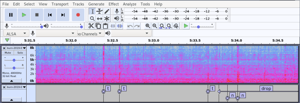
Annotating datasets
You might want to do your own dataset right. Audacity is a nice editor for for audio and it has a nice support for annotating by adding a label track.
There’s keyboard shortcuts for for all the functions that you need, so it’s quite quick to use.
So here I’m annotating some custom audio where we did event recognition
and the nice thing is that the format that they have is basically a CSV file.
It has no header and so on, but this Pandas one-liner will basically give you a nice data frame with all your annotations from the sound.
Summary
Time to summarize. We went through the basic audio pipeline.
We split the audio into fixed length analysis windows.
We used log mel-spectrogram as a sound representation because it’s shown to work very well.
We then applied a machine learning model, typically a Convolutional Neural Network.
And then we aggregated the predictions from each individual window and we merged them together using global mean pooling.
And for models I would recommend if you trying some new data,
try audio embeddings with OpenL3 and a simple model like notice fire or or random forest for instance.
Try convolutional neural network using transfer learning.
It’s quite powerful and there are usually examples that will get you pretty far.
If you do for instance preprocess spectrograms and save them as PNG files basically you can kind of take any image classification Python code that you have already.
or if you’re willing to kind of ignore this merging of different analysis windows and use that.
Data augmentation is very effective. Time-shift, time-stretch, pitch-shift, noise-add or basically recommended to use.
Sadly there is not such nice like or like go-to implementations of these in infants and Keras generators but it’s not that hard to do.
Some more learning resources for you.
The slides and also a lot of my notes in general are on this Github.
If you want a hands-on experience Tensorflow has a pretty nice tutorial called Simple Audio Recognition about recognizing speech commands.
Which could be an interesting application, but it’s taking a general approach, it’s not speech specific, so you can use it for other things.
Also there’s one book recommendation: Computational Analysis of Sound Scenes and Events.
It’s quite thorough when it comes to general audio classification. A very modern book from 2018.
Questions and Answers
Q.
Hey yeah thanks Jon, a very interesting application of machine learning. I have two questions.
So there’s obviously a like a time series component to your data, I’m not so familiar with this audio classification problem, but alright can you tell us a bit about time series methods maybe LSTM and so on how successful they are?
A.
Yes yeah time series is intuitively one would really want to apply that because there is definitely time component.
So Convolutional Recurrent Neural Networks do quite well when you’re looking at longer time scales.
For instance there’s a classification task called Audio Scene Recognition for instance.
I have a 10 or maybe 30-second clip is this from a restaurant or from a city and so on.
And there you see that the recurrent networks that do have a much stronger time modelling they do better.
But for small short tasks who CNN’s do just fine, surprisingly okay.
Q.
And the other small question I had was just to understand your label, the target that it’s learning.
You said that this is all very mixed the sound is a very mixed data set, so are the labels just like one category of sound when you’re learning,
or would it be beneficial to have you know maybe a weighted set of two categories when doing learning?
A.
Yep, so in ordinary classification tasks the typical style, or kind of by definition, is to have a single label on a some sort of window of time.
You can have multi-label datasets of course and in practice that’s a more realistic modeling of the world, because you basically always have multiple sounds.
So I think AudioSet has multi labeling and there’s a new Urbansound data set now that also has multiple labels.
And then you apply like kind of more tagging approaches.
But you’re still using classification as a base with tagging:
you can either use separate classifier per track of sound of interest,
or you can have a joint model which has multi-label classification.
So definitely this is something that you would want to do but it does complicate the problem.
Q.
You mentioned about data argumentation that we can apply Mixup to separate classes and mix them, and then the label of that mix should be weighted also because it kind of concludes with previous question usually like 0.5 and 0.5 for the other and
A.
Yes so Mixup, it was proposed things like 2-3 years ago, there’s a general method.
So you basically take your sound with your target class and you say okay let’s take 80% of that (not 100%), and then take 20% of some other sound which is a non-target class, mix it together and then update the labels accordingly.
So it’s kind of just telling you hey there is this predominant sound, but there’s also this sound in the background.
Q.
Yes you mentioned about the main frequency ranges but usually when you record audio microphones you get up to 20 thousand Hertz,
so they have you any experience or I could comment on when you have added information of the higher frequency ranges does that affect the machine learning algorithm or yeah.
A.
So typically recordings are done at 44 kilohertz or 48 kilohertz for general audio.
Often machine learning is applied at lower frequency, so with 22 kilohertz or something it is just 16, in the rare case is also 8.
So it depends on the sounds of interest if you’re doing birds definitely you want to keep that those high-frequency things.
If you’re doing speech you can do just fine on 8 kilohertz.
Usually another thing is that noise tends to be in the lower areas of the spectrum, there’s more energy in the lower end of the spectrum.
So if you are doing birds you might want to just ignore everything below 1 kilohertz for instance and that definitely simplifies your model especially if you have a small data set.
Q.
Quick question you mentioned the editor that has support for annotating audio could you please repeat the name?
A.
Yes, Audacity.
Q.
And my general question do having tips if for example you don’t have an existing dataset just starting with a bunch of audio that you want to annotate first.
Do you have any advice for strategies like some maybe semi-supervised?
A.
Yeah semi-supervised is very interesting. There’s a lot of papers but I haven’t seen like very good like practical methodology for it.
And I think in general annotating a data set is it like a whole other talk here, but I’m very interested to come to chat about this later.
Q.
Thanks to you and very nice talk.
My question would be do you have to deal with any pre-processing or like white noise filtering you mean to remove white noise,
it’s exactly just you just said like removing or ignoring certain amount?
A.
Yes, you can. I mean, scoping your frequency range definitely, it’s very easy so just do it if you if you know where your things of interests are.
Denoising. You can apply a separate denoising step beforehand and then do machine learning.
If you don’t have a lot of data, that can be very beneficial.
For instance, maybe you can use a standard denoising algorithm trained on like thousands of hours of stuff, or just a general DSP method.
If you have a lot of data then in practice the machine learning algorithm itself learns to suppress the noise.
But it only works if you have a lot of data.
Q.
So thank you for the talk.
Is it possible to train a deep convolutional neural net directly on the time domain data using a 1d convolutions and dilated convolution?
A.
Yes this is possible, and it is very actively researched.
But it’s only within the last like year or two that they’re getting to the same level of performance as spectrogram-based models.
But some models now are showing actually better performance with the end-to-end trained model
So I expect that in a couple of years maybe that will be the kind of go-to for a practical applications.
Q.
Can I do a speech recognition with this? This is only like six classes like and I think you have much more classes in speech?
A.
Yes if you want to do Automatic Speech Recognition, so the complete vocabulary of English for instance, then you can theoretically.
But there are specific models for all automatic speech recognition that will in general do better.
So if you want full speech recognition you should look at speech specific methods and there are many available.
But if you’re doing a simple task, like commands: yes/no up,down, one, two, three, four, five – you can limit your vocabulary to say maybe under a hundred classes or something, then it gets much more realistic to apply a kind of speech-unaware model like this.
Q.
Thanks for an interesting presentation.
I was just wondering from the thesis, it looks like you applied this model to a microprocessor.
Can you tell a little bit about the framework you use where you transfer it from a Python?
A.
Yes, so we use the vendor provided library from ST microelectronics for the STM32 and it’s called X-CUBE-AI.
You’ll find links in the Github.
It’s a proprietary solution, only works on that microcontroller, but it’s very simple: you throw in the Keras model, it will give you a C model out.
And they have code examples about the audio pre-processing (yeah with some bugs, but it does work).
And the firmware code for thesis is also in the Github repository, not just the model, so you can basically download that and and start going.
Over 8 years ago I completed a Bachelor in Electronics Engineering, with a focus on embedded systems. Since then I have done primarily software engineering in embedded and web projects, sometimes combined in so-called “Internet of Things” (IoT) projects. Often there was a strong data- and signal-processing focus in these systems; from audio processing in microphone-arrays, to image processing for smart website builders. Recognizing the importance of data, I realized around 2 years ago I wanted to add a new skill-set to my engineering capabilities: Data Analysis and Machine Learning (ML).
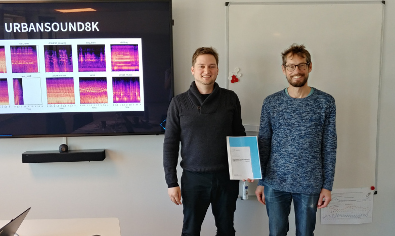
And today I’m proud to say that I have successfully completed the Master in Data Science program at the Norwegian University of Life Sciences, as one the first batch to have this degree in Norway.
Master of Data Science thesis successfully defended. Left: me, Right: External sensor Lars Erik Solheim
Research
Throughout my degree, I’ve kept the vast majority of my notes in the open-source way – public on Github. Over time I have distilled these into two resources covering the main topics of my work.
Embedded Machine Learning: Machine Learning applied to Embedded System, with a focus on-edge ML in low-cost, low-power sensors.
Machine Hearing: Using Machine Learning on audio, with a focus on general sound (less music and speech).
Thesis
My masters thesis combined these two topics, and applied it to classification of everyday urban sounds for noise monitoring in smart cities. The report and all the code can be found on Github:
Since Embedded Machine Learning is an emerging niche, the availability of software tools are not as good as for machine learning in general. To help with that I developed emlearn, an open-source ML inference engine tailored for micro-controllers and very small embedded systems. emlearn allows to convert models built with existing Python machine learning frameworks such as scikit-learn and Keras, and execute them on device using portable C code. The focus is on simple and efficient models such as Random Forests, Decision Trees, Naive Bayes, linear models. In this way, emlearn is a compliment to deep learning inference libraries for embedded devices, such as TFLite and X-CUBE-AI.
Consulting
While the master degree was nominally a full time program, I kept doing engineering work for customers in the period. Projects have included:
dlock. A IoT doorlock system for retrofitting existing public infrastructure doors. Developed for municipality of Oslo as part of the Oslonøkkelen project, an app that allows inhabitants to access municipality services such as libraries and recycling stations outside of manned working-hours. Made in collaboration with IoT solutions provider Trygvis IO.
Since the start of this year, I have started to focus on machine learning projects. Especially things that incorporate my particular expertise: Embedded/Edge Machine Learning, Machine Learning for Audio, and Machine Learning on IoT sensor data. The first ML consulting project for Roest coffee is well underway (details to be announced). Going forward, most of my time is dedicated to products at my new startup, Soundsensing. However, there should also be some capacity for new consulting work.